Photosynthesis In Plants: The Role Of Chlorophyll In Photosynthesis

Chlorophyll

Green pigments found in plants, algae and bacteria

"Leaf green" redirects here. For the RAL color, see RAL 6002 Leaf green

Chlorophyll at different scales Chlorophyll is responsible for the green color of many plants and algae. Seen through a microscope, chlorophyll is concentrated within organisms in structures called chloroplasts – shown here grouped inside plant cells. [1] Plants are perceived as green because chlorophyll absorbs mainly the blue and red wavelengths but green light, reflected by plant structures like cell walls, is less absorbed. magnesium There are several types of chlorophyll, but all share the chlorin ligand which forms the right side of this diagram.

Chlorophyll (also chlorophyl) is any of several related green pigments found in cyanobacteria and in the chloroplasts of algae and plants.[2] Its name is derived from the Greek words χλωρός, khloros ("pale green") and φύλλον, phyllon ("leaf").[3] Chlorophyll allow plants to absorb energy from light.

Chlorophylls absorb light most strongly in the blue portion of the electromagnetic spectrum as well as the red portion.[4] Conversely, it is a poor absorber of green and near-green portions of the spectrum. Hence chlorophyll-containing tissues appear green because green light, diffusively reflected by structures like cell walls, is less absorbed.[1] Two types of chlorophyll exist in the photosystems of green plants: chlorophyll a and b.[5]

History

Chlorophyll was first isolated and named by Joseph Bienaimé Caventou and Pierre Joseph Pelletier in 1817.[6] The presence of magnesium in chlorophyll was discovered in 1906,[7] and was that element's first detection in living tissue.[8]

After initial work done by German chemist Richard Willstätter spanning from 1905 to 1915, the general structure of chlorophyll a was elucidated by Hans Fischer in 1940. By 1960, when most of the stereochemistry of chlorophyll a was known, Robert Burns Woodward published a total synthesis of the molecule.[8][9] In 1967, the last remaining stereochemical elucidation was completed by Ian Fleming,[10] and in 1990 Woodward and co-authors published an updated synthesis.[11] Chlorophyll f was announced to be present in cyanobacteria and other oxygenic microorganisms that form stromatolites in 2010;[12][13] a molecular formula of C 55 H 70 O 6 N 4 Mg and a structure of (2-formyl)-chlorophyll a were deduced based on NMR, optical and mass spectra.[14]

Photosynthesis

a ( blue ) and b ( red ) in a solvent. The spectra of chlorophyll molecules are slightly modified in vivo depending on specific pigment-protein interactions. Chlorophyll A Chlorophyll B Absorbance spectra of free chlorophyll) and) in a solvent. The spectra of chlorophyll molecules are slightly modifieddepending on specific pigment-protein interactions.

Chlorophyll is vital for photosynthesis, which allows plants to absorb energy from light.[15]

Chlorophyll molecules are arranged in and around photosystems that are embedded in the thylakoid membranes of chloroplasts.[16] In these complexes, chlorophyll serves three functions:

The function of the vast majority of chlorophyll (up to several hundred molecules per photosystem) is to absorb light. Having done so, these same centers execute their second function: The transfer of that energy by resonance energy transfer to a specific chlorophyll pair in the reaction center of the photosystems. This specific pair performs the final function of chlorophylls: Charge separation, which produces the unbound protons (H+) and electrons (e−) that separately propel biosynthesis.

The two currently accepted photosystem units are photosystem I and photosystem II, which have their own distinct reaction centres, named P700 and P680, respectively. These centres are named after the wavelength (in nanometers) of their red-peak absorption maximum. The identity, function and spectral properties of the types of chlorophyll in each photosystem are distinct and determined by each other and the protein structure surrounding them.

The function of the reaction center of chlorophyll is to absorb light energy and transfer it to other parts of the photosystem. The absorbed energy of the photon is transferred to an electron in a process called charge separation. The removal of the electron from the chlorophyll is an oxidation reaction. The chlorophyll donates the high energy electron to a series of molecular intermediates called an electron transport chain. The charged reaction center of chlorophyll (P680+) is then reduced back to its ground state by accepting an electron stripped from water. The electron that reduces P680+ ultimately comes from the oxidation of water into O 2 and H+ through several intermediates. This reaction is how photosynthetic organisms such as plants produce O 2 gas, and is the source for practically all the O 2 in Earth's atmosphere. Photosystem I typically works in series with Photosystem II; thus the P700+ of Photosystem I is usually reduced as it accepts the electron, via many intermediates in the thylakoid membrane, by electrons coming, ultimately, from Photosystem II. Electron transfer reactions in the thylakoid membranes are complex, however, and the source of electrons used to reduce P700+ can vary.

The electron flow produced by the reaction center chlorophyll pigments is used to pump H+ ions across the thylakoid membrane, setting up a proton-motive force a chemiosmotic potential used mainly in the production of ATP (stored chemical energy) or to reduce NADP+ to NADPH. NADPH is a universal agent used to reduce CO 2 into sugars as well as other biosynthetic reactions.

Reaction center chlorophyll–protein complexes are capable of directly absorbing light and performing charge separation events without the assistance of other chlorophyll pigments, but the probability of that happening under a given light intensity is small. Thus, the other chlorophylls in the photosystem and antenna pigment proteins all cooperatively absorb and funnel light energy to the reaction center. Besides chlorophyll a, there are other pigments, called accessory pigments, which occur in these pigment–protein antenna complexes.

Chemical structure

a molecule Space-filling model of the chlorophyllmolecule

Several chlorophylls are known. All are defined as derivatives of the parent chlorin by the presence of a fifth, ketone-containing ring beyond the four pyrrole-like rings. Most chlorophylls are classified as chlorins, which are reduced relatives of porphyrins (found in hemoglobin). They share a common biosynthetic pathway with porphyrins, including the precursor uroporphyrinogen III. Unlike hemes, which contain iron bound to the N4 center, most chlorophylls bind magnesium. The axial ligands attached to the Mg2+ center are often omitted for clarity. Appended to the chlorin ring are various side chains, usually including a long phytyl chain (C 20 H 39 O). The most widely distributed form in terrestrial plants is chlorophyll a. The only difference between chlorophyll a and chlorophyll b is that the former has a methyl group where the latter has a formyl group. This difference causes a considerable difference in the absorption spectrum, allowing plants to absorb a greater portion of visible light.

The structures of chlorophylls are summarized below:[17][18]

Structures of chlorophylls

chlorophyll a

chlorophyll b

chlorophyll c 1

chlorophyll c 2

chlorophyll d

chlorophyll f

Measurement of chlorophyll content

Chlorophyll forms deep green solutions in organic solvents.

Chlorophylls can be extracted from the protein into organic solvents.[19][20][21] In this way, the concentration of chlorophyll within a leaf can be estimated.[22] Methods also exist to separate chlorophyll a and chlorophyll b.

In diethyl ether, chlorophyll a has approximate absorbance maxima of 430 nm and 662 nm, while chlorophyll b has approximate maxima of 453 nm and 642 nm.[23] The absorption peaks of chlorophyll a are at 465 nm and 665 nm. Chlorophyll a fluoresces at 673 nm (maximum) and 726 nm. The peak molar absorption coefficient of chlorophyll a exceeds 105 M−1 cm−1, which is among the highest for small-molecule organic compounds.[24] In 90% acetone-water, the peak absorption wavelengths of chlorophyll a are 430 nm and 664 nm; peaks for chlorophyll b are 460 nm and 647 nm; peaks for chlorophyll c 1 are 442 nm and 630 nm; peaks for chlorophyll c 2 are 444 nm and 630 nm; peaks for chlorophyll d are 401 nm, 455 nm and 696 nm.[25]

Ratio fluorescence emission can be used to measure chlorophyll content. By exciting chlorophyll a fluorescence at a lower wavelength, the ratio of chlorophyll fluorescence emission at 705±10 nm and 735±10 nm can provide a linear relationship of chlorophyll content when compared with chemical testing. The ratio F 735 /F 700 provided a correlation value of r2 0.96 compared with chemical testing in the range from 41 mg m−2 up to 675 mg m−2. Gitelson also developed a formula for direct readout of chlorophyll content in mg m−2. The formula provided a reliable method of measuring chlorophyll content from 41 mg m−2 up to 675 mg m−2 with a correlation r2 value of 0.95.[26]

Biosynthesis

In some plants, chlorophyll is derived from glutamate and is synthesised along a branched biosynthetic pathway that is shared with heme and siroheme.[27][28][29] Chlorophyll synthase[30] is the enzyme that completes the biosynthesis of chlorophyll a:[31][32]

chlorophyllide a + phytyl diphosphate ⇌ {displaystyle rightleftharpoons } a + diphosphate

This converion forms an ester of the carboxylic acid group in chlorophyllide a with the 20-carbon diterpene alcohol phytol. Chlorophyll b is made by the same enzyme acting on chlorophyllide b.

In Angiosperm plants, the later steps in the biosynthetic pathway are light-dependent. Such plants are pale (etiolated) if grown in darkness. Non-vascular plants and green algae have an additional light-independent enzyme and grow green even in darkness.[33]

Chlorophyll is bound to proteins. Protochlorophyllide, one of the biosynthetic intermediates, occurs mostly in the free form and, under light conditions, acts as a photosensitizer, forming free radicals, which can be toxic to the plant. Hence, plants regulate the amount of this chlorophyll precursor. In angiosperms, this regulation is achieved at the step of aminolevulinic acid (ALA), one of the intermediate compounds in the biosynthesis pathway. Plants that are fed by ALA accumulate high and toxic levels of protochlorophyllide; so do the mutants with a damaged regulatory system.[34]

Senescence and the chlorophyll cycle

The process of plant senescence involves the degradation of chlorophyll: for example the enzyme chlorophyllase (EC 3.1.1.14) hydrolyses the phytyl sidechain to reverse the reaction in which chlorophylls are biosynthesised from chlorophyllide a or b. Since chlorophyllide a can be converted to chlorophyllide b and the latter can be re-esterified to chlorophyll b, these processes allow cycling between chlorophylls a and b. Moreover, chlorophyll b can be directly reduced (via 71-hydroxychlorophyll a) back to chlorophyll a, completing the cycle.[35][36] In later stages of senescence, chlorophyllides are converted to a group of colourless tetrapyrroles known as nonfluorescent chlorophyll catabolites (NCC's) with the general structure:

These compounds have also been identified in ripening fruits and they give characteristic autumn colours to deciduous plants.[36][37]

Distribution

The chlorophyll maps show milligrams of chlorophyll per cubic meter of seawater each month. Places where chlorophyll amounts were very low, indicating very low numbers of phytoplankton, are blue. Places where chlorophyll concentrations were high, meaning many phytoplankton were growing, are yellow. The observations come from the Moderate Resolution Imaging Spectroradiometer (MODIS) on NASA's Aqua satellite. Land is dark gray, and places where MODIS could not collect data because of sea ice, polar darkness, or clouds are light gray. The highest chlorophyll concentrations, where tiny surface-dwelling ocean plants are thriving, are in cold polar waters or in places where ocean currents bring cold water to the surface, such as around the equator and along the shores of continents. It is not the cold water itself that stimulates the phytoplankton. Instead, the cool temperatures are often a sign that the water has welled up to the surface from deeper in the ocean, carrying nutrients that have built up over time. In polar waters, nutrients accumulate in surface waters during the dark winter months when plants cannot grow. When sunlight returns in the spring and summer, the plants flourish in high concentrations.[38]

Culinary use

Synthetic chlorophyll is registered as a food additive colorant, and its E number is E140. Chefs use chlorophyll to color a variety of foods and beverages green, such as pasta and spirits. Absinthe gains its green color naturally from the chlorophyll introduced through the large variety of herbs used in its production.[39] Chlorophyll is not soluble in water, and it is first mixed with a small quantity of vegetable oil to obtain the desired solution.[citation needed]

Biological use

A 2002 study found that "leaves exposed to strong light contained degraded major antenna proteins, unlike those kept in the dark, which is consistent with studies on the illumination of isolated proteins". This appeared to the authors as support for the hypothesis that "active oxygen species play a role in vivo" in the short-term behaviour of plants.[40]

See also

Bacteriochlorophyll, related compounds in phototrophic bacteria

Chlorophyllin, a semi-synthetic derivative of chlorophyll

Deep chlorophyll maximum

Chlorophyll fluorescence, to measure plant stress

Factors Influencing Leaf Chlorophyll Content in Natural Forests at the Biome Scale

Chlorophyll (Chl) is an important photosynthetic pigment to the plant, largely determining photosynthetic capacity and hence plant growth. However, this concept has not been verified in natural forests, especially at a large scale. Furthermore, how Chl varies in natural forests remains unclear. In this study, the leaves of 823 plant species were collected from nine typical forest communities, extending from cold-temperate to tropical zones in China, to determine the main factors influencing leaf chlorophyll content in different regions and at different scales. We measured chlorophyll a (Chl a ), chlorophyll b (Chl b ), Chl (Chl a +Chl b ), and the ratio of Chl a and Chl b (Chl a/b ). The results showed that Chl a , Chl b , and Chl a/b values were in the range of 0.87–15.92 mg g −1 (mean: 4.18 mg g −1 ), 0.32–6.42 mg g −1 (mean 1.72 mg g −1 ), and 1.43–7.07 (mean: 2.47). The values of these three Chl parameters significantly differed among plant functional groups (trees < shrubs < herbs, coniferous trees < broadleaved trees, and evergreens < deciduous trees). Unexpectedly, Chl a , Chl b , and Chl a + b increased slightly with increasing latitude. Climate, soil, and phylogeny exert only a small effect on the spatial variation of Chl in natural forests, with large variation in the Chl of coexisting species masking the spatial patterns. This study is the first to report variations in Chl among different types of natural forests at a large scale, demonstrating that the fuzzy regulation of Chl makes it very difficult to take Chl as the main input parameter to the models of natural forests.

Introduction

Photosynthesis is the most important source of energy for plant growth (Mackinney, 1941; Baker, 2008), because chlorophyll (Chl) represents an important pigment for photosynthesis. The photosynthetic reaction is mainly divided into three steps: (1) primary reaction, (2) photosynthetic electron transport and photophosphorylation, and (3) carbon assimilation. Chlorophyll a (Chl a) and chlorophyll b (Chl b) are essential for the primary reaction. Chl a and Chl b absorb sunlight at different wavelengths (Chl a mainly absorbs red-orange light and Chl b mainly absorbs blue-purple light), leading to the assumption that the total amount leaf chlorophyll content (Chl a+b) and allocated ratio (Chl a/b) directly influence the photosynthetic capacity of plants. This assumption has been verified by a controlled experiment using several plant species (Croft et al., 2017). However, to date, it is unclear how leaf Chl content varies among plant species, plant functional groups (PFGs), and communities in natural forests, especially at a large scale.

When considering on the importance of Chl for photosynthesis, plants in the natural community should optimize light absorption and photosynthesis by adjusting the content and ratios of Chl to enhance growth and survival at the long-term evolutionary scale. Certain factors might influence Chl levels. From the perspective of phylogeny, stable traits are the results of long-term adaption and evolution to the external environments. If Chl was a stable trait, the length of evolutionary history should have a constraining effect on it. In other words, Chl should be influenced by phylogeny. Some studies have demonstrated that phyletic evolution significantly influences certain leaf traits, such as element content and wood traits (He et al., 2010; Zhang et al., 2011; Liu et al., 2012; Zhao et al., 2014). If Chl is really influenced by phylogeny, the rule of Chl should be used only after excluding phylogenetic effects by using phylogenetically independent contrasts in future studies.

Alternatively, plants inevitably adjust their own traits to adapt to different environments. Therefore, it is widely considered that plants should adjust Chl (Chl a, Chl b, Chl a+b, and Chl a/b) to adapt to a given environment and optimize photosynthesis. Thus, climate and soils should play important roles in regulating Chl, especially at a large scale. Chlorophyll synthesis requires many elements nitrogen (N), phosphorous (P)] from soils; thus, soils should influence Chl (Fredeen et al., 1990). The synthesis of chlorophyll needs through a series of enzymatic reactions, with the temperatures that are too high or low inhibiting the enzyme reaction, even destroying the original chlorophyll. The optimum temperature of general plant chlorophyll synthesis is 30°C, DVR enzyme activity peaking at 30°C (Nagata et al., 2005). Thus, temperature also influences chlorophyll synthesis (Wolken et al., 1955). Precipitation might affect the photochemical activity of chloroplasts (Zhou, 2003), with water being the medium used for transporting nutrients in plants, as mineral salts must be dissolved in water to be absorbed by plants. Consequently, chlorophyll synthesis and water are closely related. The lack of water in leaves influences the synthesis of chlorophyll and promotes the decomposition of chlorophyll, and accelerating leaf yellowing. There is also indirect evidence that Chl is jointly controlled by climate and soils; thus, Chl might be an indicative trait for characterizing how plants respond to climate change.

A major challenge is establishing how to link traits and functioning in natural ecosystems; yet, such knowledge is important to predict how ecosystem functioning varies with changing environments (Garnier and Navas, 2012; Reichstein et al., 2014). Because of the importance of Chl on photosynthesis, scientists assumed that a relationship between Chl and gross primary production (GPP) exists, using this relationship for model optimization. For instance, Croft et al. (2017) found that, for several plant species, it is better to use Chl as a proxy to replace photosynthetic efficiency, than the traditional substitute-leaf N content, when establishing models of GPP in forest communities. This approach was innovative and exciting for scientists involved in physiological ecology and macroecology. The reliability of leaf Chl content represents the maximum rate of carboxylation (V max ), and has the potential for use as a proxy in models in the future (Croft et al., 2017). However, it is difficult to obtain data on Chl in natural communities, especially at a large scale.

In this study, we investigated Chl across 823 plant species from nine forests, extending from tropical forests to cold-temperate forests in eastern China. Using these data, we explored variation in Chl, latitudinal patterns, and underlying influencing factors (climate, soil, and phylogeny). The main objectives of this study were to: (1) investigate how Chl varies in natural forests among different plant species, PFGs, and communities; (2) determine whether there is a latitudinal pattern in Chl; (3) identify the main factors influencing Chl (phylogeny, climate, and soil); and (4) provide large-scale evidence supporting the concept that Chl is a reliable proxy of V max in global ecological models.

Materials and Methods

Site Description

The North-South Transect of Eastern China (NSTEC) is the fifteenth standard transect of the International Geosphere-Biosphere Program(IGBP), which is a unique forest belt mainly driven by thermal gradient and encompasses almost all forest types found in the northern hemisphere (Canadell et al., 2002). In this study, nine natural forests along the NSTEC were selected along the 4,200-km transect, including: Jiangfeng (JF), Dinghu (DH), Jiulian (JL), Shennong (SN), Taiyue (TY), Dongling (DL), Changbai (CB), Liangshui (LS), and Huzhong (HZ) (Figure S1). These nine forests span cold-temperate, temperate, subtropical, and tropical forests from 18.7 to 51.8°N. The mean annual temperature (MAT) of these forests ranges from −4.4 to 20.9°C, while mean annual precipitation (MAP) ranges from 481.6 to 2449.0 mm. Soils vary from tropical red soils with low organic matter to brown soils with high organic matter (Song et al., 2016). Detailed geographical information of the region is presented in Table S1.

Field Sampling

The field survey was conducted between July and August of 2013. First, four experimental plots (30 × 40 m) were selected in each forest. The geographical details, plant species composition, and community structure were determined for each plot. Trees were measured within the 30 × 40 m plots. Next, four quadrats (5 × 5 m) of shrubs and four plots (1 × 1 m) of herbs were setup at the four corners of each experimental plot. All common species were identified in each plot, including trees, shrubs, and herbs. Subsequently, we collected more than 30 pieces of leaves from each species, of which four pieces were randomly selected to cut up and determine chlorophyll content from each plant species within the plot. We chose mature and healthy trees, and collected fully expanded, sun-exposed leaves from four individuals of each plant species, which were considered as four repetitions (Zhao et al., 2016). Overall, the leaves of 823 plant species were collected. Soil samples (0–10 cm depth) were randomly collected from 30 to 50 points using a soil sampler (6-cm diameter) in each plot and were combined to form one composite sample in each plot (Tian et al., 2016; Wang et al., 2016; Li et al., 2018).

Measurement of Leaf Chlorophyll Content

Fresh leaves were cleaned to remove soil and other contaminants, and 0.1 g of fresh leaves was used to extract chlorophyll using 95% ethanol, with four replicates for each species of plants. The Chl content (Chl a and Chl b) of the filtered solution was measured using the classical spectrophotometric method with a spectrophotometer (Pharma Spec, UV-1700, Shimadzu, Japan) (Mackinney, 1941; Li et al., 2018).

According to the Lambert-Beer law, the relationship between concentration and optical density is:

D 665 = 83 . 31 C a + 18 . 60 C b ( 1 )

D 649 = 4 . 54 C a + 44 . 24 C b ( 2 )

G = C a + C b ( 3 )

where D 665 and D 649 are the optical densities of the chlorophyll solution at wavelengths 665 and 649 nm; C a , C b , and G are the concentrations of Chl a, Chl b, and total Chl, respectively (g L−1); 83.31 and 18.60 are the specific absorption of Chl a and Chl b at a wavelength of 665 nm; and 24.54 and 44.24 are the specific absorption of Chl a and Chl b at a wavelength of 649 nm.

Chl a ( mg g - 1 ) = C a × 50 / ( 1000 × 0 . 1 ) ( 4 )

Chl b ( mg g - 1 ) = C b × 50 / ( 1000 × 0 . 1 ) ( 5 )

Then, Chl a+b and Chl a/b were calculated (mg g−1, leaf fresh mass, FM) as:

Chl a + b ( mg g - 1 ) = G × 50 / ( 1000 × 0 . 1 ) ( 6 )

Chl a / b = Chl a Chl b ( 7 )

Measurement of Soil Parameters

Soil samples were acidified with HNO 3 and HF overnight. Then, the samples were digested using a microwave digestion system (Mars X Press Microwave Digestion system, CEM, Matthews, NC, USA) before analyzing soil total phosphorus (STP) content.

Elemental analyzer (Vario Analyzer, Elementar, Germany) was used to measure soil organic carbon (SOC) and soil total nitrogen (STN). Soil pH was determined using a pH meter (Mettler Toledo Delta 320, Switzerland) by using a slurry of soil and distilled water (1: 2.5) (Zhao et al., 2014).

Climate Data

The primary climate variables, including mean annual temperature (MAT) and mean annual precipitation (MAP), were extracted from the climate dataset at a 1 × 1 km spatial resolution. The data were collected at 740 climate stations of the China Meteorological Administration, from 1961 to 2007, using the interpolation software ANUSPLIN (He et al., 2014).

Phylogeny

Eight hundred and twenty-three species of plants were used to construct a phylogenetic tree at the species and family levels. First, we checked the species information in the Plant List and confirmed the correct Latin names of each species. Second, we defined a reference phylogenetic tree by using the “phytools” package in R and S. Phylo Maker (Qian and Jin, 2016), and generated the phylogenetic tree in the MAGA 5.1. Finally, using the algorithm BLADJ provided by the software Phylocom (Webb et al., 2008), according to molecular and fossil dating data (Wikström et al., 2001), we calculated the time of each node in the phylogenetic tree (in one million, m letters years, MY). At the family level, according to the evolution of angiosperm families provided by molecular and fossil dating data, we identified the evolution of angiosperm families.

Statistical Analysis

Plant species were divided by plant functional groups (PFGs, trees, shrubs, and herbs), growth forms (coniferous or broadleaved tree), and leaf types (evergreen or deciduous tree). One–way analysis of variance (ANOVA) with the post-hoc Duncan's multiple comparison was used to test the differences in Chl for different sites, PFGs, and leaf types. We used regression analyses to explore latitudinal patterns of Chl. To analyze the factors influencing Chl, we calculated Spearman's rank correlation coefficients for 823 plant species across sites, PFGs, and leaf types. We then used redundancy analysis (RDA) to analyze the relative influences of climate, soil, and the interspecific variation of species.

The strength of the phylogenetic signal in Chl a, Chl b, Chl a+b, Chl a/b across plant species was quantified using Blomberg's K statistics, which tests whether observed traits vary across a phylogeny (Blomberg et al., 2003). We tested the significance of this phylogenetic signal by comparing the actual system to a null model without phylogenetic structure. If the real value of the phylogenetic signal in the trait was greater than 95% that of the null model (P < 0.05), the phylogenetic signal was considered significant, and vice versa. The phylogenetic signal was quantified and tested using the “picante” package in R.

All analyses were conducted using the software SPSS 17.0 (SPSS Inc., Chicago, IL, USA) or R (version 3.3.1, R Development Core Team). All figures were produced in Sigma Plot 10.0 (Washington, IL, USA, 2006). The significance level was set at P < 0.05.

Results

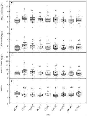
Across the 823-plant species, Chl a, Chl b, Chl a+b, and Chl a/b showed unimodal distributions in each type of forest (Figure 1). Chl a ranged from 0.87 to 15.92 mg g−1, with an average of 4.18 mg g−1; Chl b ranged from 0.32 to 6.42 mg g−1, with an average of 1.72 mg g−1; Chl a+b ranged from 1.20 to 22.58 mg g−1, with an average of 5.97 mg g−1; and Chl a/b ranged from 0.87 to 15.92, with an average of 2.47. Coefficient of variations of Chl a, Chl b, Chl a+b, and Chl a/b were 0.41, 0.43, 0.41, and 0.14, respectively (Table 1). There were significant differences in Chl a, Chl b, Chl a+b, and Chl a/b among different communities (P < 0.05) (Figure 1, Table S2). Chl was significant in different PFGs and life forms, with trees > shrubs > herbs, evergreens > deciduous trees, broadleaved > conifers on Chl a, Chl b, and Chl a+b; trees < shrubs < herbs, conifers < broadleaved on Chl a/b (Tables 1–3). However, no significant difference between evergreens and deciduous trees was observed for Chl a/b.

FIGURE 1

Figure 1. Statistics of leaf chlorophyll content for the nine study forests along the North-South Transect of Eastern China (NSTEC). (A–D) were calculated in Chl a, Chl b, Chl a+b, Chl a/b, respectively. The black lines across the boxes are median values and red points represent the means. HZ, Huzhong; LS, Liangshui; CB, Changbai; DL, Dongling; TY, Taiyue; SN, Shennongjia; JL, Jiulian; DH, Dinghu; JF, Jianfengling. Numbers in brackets represent the number of sample species in the specific site. Same letters denote no significant difference among the nine sites (P < 0.05).

TABLE 1

Table 1. Statistics of leaf chlorophyll content (mg g−1) for different life forms in forests.

TABLE 2

Table 2. Statistics of leaf chlorophyll content (mg g−1) for different growth forms in forests.

TABLE 3

Table 3. Statistics of leaf chlorophyll content (mg g−1) for different leaf shapes in forests.

To quantify the variance of different groups (sites, life forms), interpretation ratios were calculated within groups and among groups. The variance of Chl a, Chl b, Chl a+b, and Chl a/b was mainly explained by within-site variation, with only a small portion arising from among-site variation (Figure 2A). Similar results were obtained for different plants with respect to life forms and leaf types (Figures 2B–D). Chl a, Chl b, and Chl a+b increased with increasing latitude; however, this trend was weak (all Ps < 0.01, R2 = 0.02) (Figures 3A–C). In comparison, there was not obvious latitudinal pattern on Chl a/b (Figure 3D). The contents of Chl a, Chl b, and Chl a+b in leaves were negatively correlated with MAT and MAP (all P's < 0.01), and no significant relationships between Chl a/b and both MAT and MAP were observed (Figures S2, S3).

FIGURE 2

Figure 2. Partitioning the total spatial variance of leaf chlorophyll content in the nine forests (A), different life forms (B), different growth forms (C), and different leaf shapes (D).

FIGURE 3

Figure 3. Latitudinal trends of leaf chlorophyll traits in the forests of China. (A–D) were calculated in Chl a, Chl b, Chl a+b, Chl a/b, respectively. Only significant regression (P < 0.05) being given. **P < 0.01.

Significant phylogenetic signals were observed for Chl a within life forms, communities, and across the whole transect, except for shrubs and conifer trees (Table 4). The K-values were approximately equal to 0. Significant phylogenetic signals were observed for Chl b within life forms and communities, and across the whole transect, except for shrubs and conifer trees. K-values were approximately equal to 0. There were no significant phylogenetic signals in Chl a/b (Table 4). Across different sites, there were no significant phylogenetic signals in Chl a+b at most sites (Table 5). Significant phylogenetic signals were observed for Chl a+b at some sites; however, all K-values were approximately equal to 0. In other words, the phylogenetic signals were too weak for Chl a, Chl b, Chl a+b, and Chl a/b (Figures S4, S5).

TABLE 4

Table 4. Strength of the phylogenetic signal in chlorophyll traits for different growth forms.

TABLE 5

Table 5. Strength of the phylogenetic signal in chlorophyll traits for each of the nine forests.

Across all species, Chl a was negatively correlated with MAT and MAP (Ps < 0.01) and positively correlated with SOC, STN, and STP (Ps < 0.01). Chl b and Chl a+b were negatively correlated to MAT and MAP (Ps < 0.01), and positively correlated to SOC, STN, and STP. Chl a/b was negatively correlated to SOC and STP (Table S3). Environmental factors affected the Chl of PFGs and leaf types differently (Tables S4–S6). Environmental factors had weak influences on Chl a, Chl b, Chl a+b, and Chl a/b. Furthermore, more than 80% of the total variation of Chl a, Chl b, and Chl a+b could be explained by the interspecific variation in different life forms, forest communities, except for shrubs and conifer trees. For conifer trees, these Chl parameters explained 45% of variation. The contributions of climate and soil factors to the total variance of Chl along the transect were very low, less than 1% for all parameters (Table S7).

Discussion

Significant Differences in Chl Among Different Species, Life Forms, and Communities

Large variation in Chl was observed among the 823-plant species in the natural forest communities. Across all plants, there were significant differences of Chl among different species, life forms, and communities. The coefficient of variations of Chl a, Chl b, Chl a+b, and Chl a/b were 0.41, 0.43, 0.41, and 0.14, respectively. The coefficient of variations of Chl a/b was relatively smaller than that of Chl a, Chl b, and Chl a+b. Although interspecific differences in Chl a and Chl b were very big, there should be a strong linear relationship between Chl a and Chl b (Li et al., 2018), lowering the variability of Chl a/b. Furthermore, the coefficients of variation of Chl a, Chl b, and Chl a+b were also large. Less than 10% of the total variation was among groups when all species were divided into diverse groups by sites, life forms, and leaf types. Especially for Chl a/b, total variation was close to zero. Interspecific variation might explain more than 80% of the total variations of Chl, which further confirms the presence of the larger interspecific variation of Chl.

Weak Increasing Latitudinal Pattern of Chl in Natural Forests

Although there were significant latitudinal patterns for Chl a, Chl b, and Chl a+b, the R2s were very weak. Chl a/b had no significant latitudinal pattern. The correlations between Chl contents and both MAT and MAP were weak. This phenomenon might be explained by a large amount of Chl in the forest communities being redundant, some of the plant chlorophyll is not involved in the photosynthetic reaction. Therefore, chlorophyll content is not necessarily linked to this reaction, even though temperature and water are the important factors in the synthesis of chlorophyll. Alternatively, high interspecific variation might have led to a weak latitudinal pattern in our study, with the highest coefficient of variation of Chl reaching 0.52. Yet, interspecific species variation could not be explained by environmental differences between the scale of the study and the observed weak latitudinal patterns. Furthermore, chlorophyll content might be affected by community structure, because the light shading effect on vertical structure might change Chl. Some control experiments found that shading effect might affect plant Chl content, and Chl a/b may also decrease.

With the development of the molecular clock theory (molecular evolution speed constancy) and fossil dating data, researchers found that phylogenic history play a decisive role for some plant traits (Comas et al., 2014; Kong et al., 2014; Li et al., 2015). Some plant traits N and P content and calorific values) are strongly affected by the phylogeny of plant species (Stock and Verboom, 2012; Chen et al., 2013; Song et al., 2016). In contrast, in our study, although Chl in the overall and different life forms had significant phylogenetic signals, the phylogenetic signal K values were close to zero. Theoretically, these traits were deemed as a strong phylogenetic signal if the K value > 1. Previous studies have demonstrated that if a plant trait has a significant phylogenetic signal, it could be considered as a conservative trait. Traits also perform more similarly when the genetic relationship of different species is closer (Felsenstein, 1985), and vice versa. Therefore, our results showed that Chl is almost not influenced by phylogeny in forests at a large scale.

In theory, as an important photosynthetic pigment of plants, Chl is widely influenced by the environment. Unexpectedly, our results showed that both climate and soil factors had very small influences on Chl, while interspecific variation was the main factor influencing the spatial patterns of Chl from tropical to cold-temperate forests. Through the redundancy analysis, we found that climate and soil factors were not the main factors influencing Chl, because their independent effects were less than 1%. However, interspecific variation did explain more than 80% of Chl. Thus, our results support that plants adapt to the environment by adjusting Chl. Because of the small plasticity of Chl, the variability of Chl in single species had a certain threshold. Above this threshold, some plants would be replaced by others because of the environmental filter. This hypothesis requires to be verified in natural forests in future. Some studies have demonstrated that the variability of leaf traits is influenced by a combination of species, climate, and soil factors (Reich et al., 2007; Han et al., 2011; Liu et al., 2012).

At a large scale, the patterns of leaf traits are not obvious along the changing environmental gradient, with greater variability occurring in species that coexist (Freschet et al., 2011; Onoda et al., 2011; Moles et al., 2014). Twenty-percent of spatial variation in leaf economic traits (specific leaf area, leaf longevity, photosynthetic rate, and leaf N and P content) is associated with the coexistence of different plant species (Wright et al., 2004; Freschet et al., 2011). Furthermore, previous control experiments showed that Chl is significantly associated with temperature and moisture (Yamane et al., 2000; Yin et al., 2006). However, the environmental factors used in this study were MAT and MAP, it would be an interesting idea to obtain the real-time data of chlorophyll and temperature and precipitation for future work. For the relationship between Chl and soil nutrients, we found that soils explain a small portion of total variation, because important elements are prioritized for important organs. As an important photosynthetic pigment, leaves should receive more nutrient elements for Chl, even if the low content of nutrient elements in soils has a small effect on Chl. Therefore, future research should focus on understanding how soils and the climate influence or optimize ecosystem functioning through a combination of element allocation. In addition, light is an important factor for chlorophyll synthesis, however in our analyzes light was not taken into account. To my knowledge, radiation could be measured using satellite data, and light extinction within forest canopies can be modeled. These would be potential next steps for our research.

Chl Should be Cautiously Used as a Proxy for Simulating GPP in Natural Communities

The main purpose of most studies on Chl in natural communities has been to establish a link between Chl and ecosystems functioning, because Chl is widely considered an important factor influencing leaf photosynthetic capacity (Singsaas et al., 2004). Using four deciduous tree species sampled across three growing seasons, Croft et al. (2017) showed that, compared with leaf N content, Chl serves as a better proxy for leaf photosynthetic capacity. Furthermore, Chl can be modeled accurately from remotely sensed data (Croft et al., 2013); thus, this important parameter has been used to model leaf photosynthetic capacity at the global scale (Jacquemoud and Baret, 1990).

However, our results showed that significant differences in Chl occur among coexisting species, functional groups, and communities. Furthermore, the vertical structure of the plant community generated strong variation in the light environment, which might result in the accumulation of redundant Chl. In addition, our previous studies have also found that Chl showed a weak correlation with GPP in the communities (Li et al., 2018). Therefore, the photosynthetic capacity in a given natural forest community could be overestimated by using Chl. In other words, when using Chl as a proxy of GPP in the natural community, the outputs should be treated with caution. While it is a clever concept to optimize models using Chl data derived through remote sensing technology, more research is required to link Chl and GPP in the natural community in a way that is both representative and informative.

Conclusions

Significant variation in Chl was observed among different plant species, functional groups, and communities. Unexpectedly, Chl showed a very weak latitudinal pattern from tropical monsoon forests to cold-temperate coniferous forests, because of significant variation among coexisting species. This interspecific variation was the main factor affecting Chl, rather than soil and climate. Because of this “fuzzy regulation” of Chl in the natural community, caution should be taken when integrating Chl in ecological models. In conclusion, this approach should only being used if scientists are able to link Chl with ecosystem functioning in natural forest communities objectively in future studies.

Authors Contributions

NH and JH conceived the ideas and designed methodology; YL, LX, CL, JZ, QW, XZ, and XW collected the data; NH and YL analyzed the data; YL, NH, and JH led the writing of the manuscript. All authors contributed critically to the drafts and gave final approval for publication.

Conflict of Interest Statement

The authors declare that the research was conducted in the absence of any commercial or financial relationships that could be construed as a potential conflict of interest.

Acknowledgments

This work was supported by the National Key Research Project of China (2017YFC0504004, 2016YFC0500202), the National Natural Science Foundation of China (31000263, 611606015, 31290221), STS of Chinese Academy of Sciences (KFJ-SW-STS-167), and the program of Youth Innovation Research Team Project (LENOM2016Q0005).

Supplementary Material

The Supplementary Material for this article can be found online at:

References

Canadell, J. G., Steffen, W. L., and White, P. S. (2002). IGBP/GCTE terrestrial transects: dynamics of terrestrial ecosystems under environmental change. J. Veg. Sci. 13, 298–300. doi: CrossRef Full Text | Google Scholar

Chen, Y., Han, W., Tang, L., Tang, Z., and Fang, J. (2013). Leaf nitrogen and phosphorus concentrations of woody plants differ in responses to climate, soil and plant growth form. Ecography 36, 178–184. doi: 10.1111/j.1600-0587.2011.06833.x CrossRef Full Text | Google Scholar

Comas, L. H., Callahan, H. S., and Midford, P. E. (2014). Patterns in root traits of woody species hosting arbuscular and ectomycorrhizas: implications for the evolution of belowground strategies. Ecol. Evol. 4, 2979–2990. doi: 10.1002/ece3.1147 PubMed Abstract | CrossRef Full Text | Google Scholar

Croft, H., Chen, J. M., Zhang, Y., and Simic, A. (2013). Modelling leaf chlorophyll content in broadleaf and needle leaf canopies from ground, CASI, Landsat TM 5 and MERIS reflectance data. Remote Sens. Environ. 133, 128–140. doi: CrossRef Full Text | Google Scholar

Freschet, G. T., Dias, A. T. C., Ackerly, D. D., Aerts, R., van Bodegom, P. M., Cornwell, W. K., et al. (2011). Global to community scale differences in the prevalence of convergent over divergent leaf trait distributions in plan asssemblages. Glob. Ecol. Biogeogr. 20, 755–765. doi: 10.1111/j.1466-8238.2011.00651.x CrossRef Full Text | Google Scholar

Garnier, E., and Navas, M. L. (2012). A trait-based approach to comparative functional plant ecology: concepts, methods and applications for agroecology. A review. Agron. Sustain. Dev. 32, 365–399. doi: 10.1007/s13593-011-0036-y CrossRef Full Text | Google Scholar

Han, W. X., Fang, J. Y., Reich, P. B., Woodward, F., and Wang, Z. (2011). Biogeography and variability of eleven mineral elements in plant leaves across gradients of climate, soil and plant functional type in China. Ecol. Lett. 14, 788–796. doi: 10.1111/j.1461-0248.2011.01641.x PubMed Abstract | CrossRef Full Text | Google Scholar

He, H., Liu, M., Xiao, X., Ren, X., Zhang, L., Sun, X., et al. (2014). Large-scale estimation and uncertainty analysis of gross primary production in Tibetan alpine grasslands. J. Geophys. Res. 119, 466–486. doi: 10.1002/2013JG002449 CrossRef Full Text | Google Scholar

He, J. S., Wang, X., Schmid, B., Dan, F. B. F., Li, X., Reich, P. B., et al. (2010). Taxonomic identity, phylogeny, climate and soil fertility as drivers of leaf traits across Chinese grassland biomes. J. Plant Res. 123, 551–561. doi: 10.1007/s10265-009-0294-9 PubMed Abstract | CrossRef Full Text | Google Scholar

Jacquemoud, S., and Baret, F. (1990). Prospect: a model of leaf optical properties spectra. Remote Sens. Environ. 34, 75–91. doi: 10.1016/0034-4257(90)90100-Z CrossRef Full Text | Google Scholar

Kong, D., Ma, C., Zhang, Q., Li, L., Chen, X., Zeng, H., et al. (2014). Leading dimensions in absorptive root trait variation across 96 subtropical forest species. New Phytol. 203, 863–872. doi: 10.1111/nph.12842 PubMed Abstract | CrossRef Full Text | Google Scholar

Li, Y., Liu, C., Zhang, J., Yao, H., Xu, L., Wang, Q., Lawren, S., et al. (2018). Variation in leaf chlorophyll concentration from tropical to cold-temperate forests: association with gross primary productivity. Ecol. Indic. 85, 383–389. doi: CrossRef Full Text | Google Scholar

Liu, C., Wang, X., Wu, X., Dai, S., He, J., and Yin, W. (2012). Relative effects of phylogeny, biological characters and environments on leaf traits in shrub biomes across central Inner Mongolia, China. J. Plant Ecol. 6, 220–231. doi: 10.1093/jpe/rts028 CrossRef Full Text | Google Scholar

Mackinney, G. (1941). Absorption of light by chlorophyll solutions. J. Biol. Chem. 140, 315–322. Google Scholar

Moles, A. T., Perkins, S. E., Laffan, S. W., Flores-Moreno, H., Awasthy, M., Tindall, M. L., et al. (2014). Which is a better predictor of plant traits: temperature or precipitation? J. Veg. Sci. 25, 1167–1180. doi: 10.1111/jvs.12190 CrossRef Full Text | Google Scholar

Nagata, N., Tanaka, R., Satoh, S., and Tanaka, A. (2005). Identification of a vinyl reductase gene for chlorophyll synthesis in Arabidopsis thaliana and implications for the evolution of Prochlorococcus species. Plant Cell 17, 233–240. doi: 10.1105/tpc.104.027276 PubMed Abstract | CrossRef Full Text | Google Scholar

Qian, H., and Jin, Y. (2016). An updated megaphylogeny of plants, a tool for generating plant phylogenies and an analysis of phylogenetic community structure. J. Plant Ecol. 9, 233–239. doi: 10.1093/jpe/rtv047 CrossRef Full Text | Google Scholar

Singsaas, E. L., Ort, D. R., and Delucia, E. H. (2004). Elevated CO 2 effects on mesophyll conductance and its consequences for interpreting photosynthetic physiology. Plant Cell Environ. 27, 41–50. doi: 10.1046/j.0016-8025.2003.01123.x CrossRef Full Text | Google Scholar

Song, G., Ying, L., Zhang, J., Li, M., Hou, J., and He, N. (2016). Significant phylogenetic signal and climate-related trends in leaf caloric value from tropical to cold-temperate forests. Sci. Rep. 6:36674. doi: 10.1038/srep36674 PubMed Abstract | CrossRef Full Text | Google Scholar

Stock, W. D., and Verboom, G. A. (2012). Phylogenetic ecology of foliar N and P concentrations and N:P ratios across mediterranean-type ecosystems. Glob. Ecol. Biogeogr. 21, 1147–1156. doi: 10.1111/j.1466-8238.2011.00752.x CrossRef Full Text | Google Scholar

Tian, M., Yu, G., He, N., and Hou, J. (2016). Leaf morphological and anatomical traits from tropical to temperate coniferous forests: mechanisms and influencing factors. Sci. Rep. 6:19703. doi: 10.1038/srep19703 PubMed Abstract | CrossRef Full Text | Google Scholar

Wang, Q., He, N., Yu, G., Gao, Y., Wen, X., Wang, R., et al. (2016). Soil microbial respiration rate and temperature sensitivity along a north-south forest transect in eastern China: patterns and influencing factors. J. Geophys. Res. 121, 399–410. doi: 10.1002/2015JG003217 CrossRef Full Text | Google Scholar

Wolken, J. J., Mellon, A. D., and Greenblatt, C. L. (1955). Environmental factors affecting growth and chlorophyll synthesis in euglena. I. physical and chemical. II. the effectiveness of the spectrum for chlorophyll synthesis. J. Eukaryot. Microbiol. 2, 89–96. Google Scholar

Yamane, Y., Shikanai, T., Kashino, Y., Koike, H., and Satoh, K. (2000). Reduction of QA in the dark: another cause of fluorescence Fo increases by high temperatures in higher plants. Photosyn. Res. 63, 23–34. doi: 10.1023/A:1006350706802 PubMed Abstract | CrossRef Full Text | Google Scholar

Yin, C., Berninger, F., and Li, C. (2006). Photosynthetic responses of Populus przewalski subjected to drought stress. Photosynthetica 44, 62–68. doi: 10.1007/s11099-005-0159-y CrossRef Full Text | Google Scholar

Zhang, S., Slik, J. W. F., Zhang, J., and Cao, K. (2011). Spatial patterns of wood traits in China are controlled by phylogeny and the environment. Glob. Ecol. Biogeogr. 20, 241–250. doi: 10.1111/j.1466-8238.2010.00582.x CrossRef Full Text | Google Scholar

Zhao, N., He, N., Wang, Q., Zhang, X., Wang, R., Xu, Z., et al. (2014). The altitudinal patterns of leaf C:N:P stoichiometry are regulated by plant growth form, climate and soil on Changbai Mountain, China. PLoS ONE 9:e95196. doi: 10.1371/journal.pone.0095196 PubMed Abstract | CrossRef Full Text | Google Scholar

Zhao, N., Yu, G., He, N., Wang, Q., Guo, D., Zhang, X., et al. (2016). Coordinated pattern of multi-element variability in leaves and roots across Chinese forest biomes: multi-element variability in leaves and roots. Glob. Ecol. Biogeogr. 25, 359–367. doi: 10.1111/geb.12427 CrossRef Full Text | Google Scholar

Photosynthesis In Plants: The Role Of Chlorophyll In Photosynthesis

What is chlorophyll and what is photosynthesis? Most of us already know the answers to these questions but for kids, this can be uncharted waters. To help kids gain a better understanding of the role of chlorophyll in photosynthesis in plants, keep reading.

What is Photosynthesis?

Plants, just like humans, require food in order to survive and grow. However, a plant’s food looks nothing like our food. Plants are the greatest consumer of solar energy, using power from the sun to mix up an energy rich meal. The process where plants make their own food is known as photosynthesis.

Photosynthesis in plants is an extremely useful process whereby green plants take up carbon dioxide (a toxin) from the air and produce rich oxygen. Green plants are the only living thing on earth that are capable of converting the sun’s energy into food.

Almost all living things are dependent upon the process of photosynthesis for life. Without plants, we would not have oxygen and the animals would have nothing to eat, and neither would we.

What is Chlorophyll?

The role of chlorophyll in photosynthesis is vital. Chlorophyll, which resides in the chloroplasts of plants, is the green pigment that is necessary in order for plants to convert carbon dioxide and water, using sunlight, into oxygen and glucose.

During photosynthesis, chlorophyll captures the sun’s rays and creates sugary carbohydrates or energy, which allows the plant to grow.

Understanding Chlorophyll and Photosynthesis for Kids

Teaching children about the process of photosynthesis and the importance of chlorophyll is an integral part of most elementary and middle school science curriculums. Although the process is quite complex in its entirety, it can be simplified enough so that younger children can grasp the concept.

Photosynthesis in plants can be compared with the digestive system in that they both break down vital elements to produce energy that is used for nourishment and growth. Some of this energy is used immediately, and some is stored for later use.

Many younger children may have the misconception that plants take in food from their surroundings, therefore, teaching them the process of photosynthesis is vital to them grasping the fact that plants actually gather the raw ingredients necessary to make their own food.

Photosynthesis Activity for Kids

Hands-on activities are the best way to teach kids how the process of photosynthesis works. Demonstrate how the sun is necessary for photosynthesis by placing one bean sprout in a sunny location and one in a dark location.

Both plants should be watered regularly. As students observe and compare the two plants over time, they will see the importance of sunlight. The bean plant in the sun will grow and thrive while the bean plant in the dark will become very sickly and brown.

This activity will demonstrate that a plant cannot make its own food in the absence of sunlight. Have children sketch pictures of the two plants over several weeks and make notes regarding their observations.